A New Way to Look at NBA Fantasy Ranking
NBA Fantasy Ranking
Project maintained by azedlee Hosted on GitHub Pages — Theme by mattgraham
Table of Contents
I. Problem statement
Yahoo, ESPN and other fantasy basketball websites are fairly inaccurate on their pre-ranking system. It is quite well known that many advanced/knowledgeable/experienced players know to never follow any of the ranking system provided by Yahoo, ESPN, etc... because they are terribly inaccurate. From research, Yahoo, ESPN and many other sites use AccuScore.com or Rotowire.com as their base ranking system. Afterwards, each website has their own fantasy "guru" that will re-arrange and edit the ranking system based on injury or potential. Third party fantasy "guru" websites also seem to work similarly, except they seem to have their own base ranking system and then edited on biased opinion (individually or a group of people). Regardless, all these websites do not have a non-biased, non-opinionated ranking system, which is understandable because ranking players correctly is extremely difficult and everyone has their own opinion on who has more potential. Currently, this seems like the best way to create a better ranking system.
My goal is to beat all their ranking systems by creating a new way to look at how people should refer to drafting. Based on the last 20 seasons, I want to create a customizable grouping system, rather than labeling players on ranks. For example, in standard leagues there are 12 managers drafting 13 players each, which means that there are 13 rounds of drafting. I want to put the 12 best players in the current pool into each round bracket, provide their mean fantasy value per season, their standard deviation and variance in all their seasons. Also, create a 14th bucket for all the other players. Based on these aspects, managers, especially new players, are able to understand what kind of player they are drafting and what kind of risks they will encounter. This, to me, is a much more accurate and effective way of drafting.
II. Description of data
All data was scraped from stats.nba.com, which is hosted by SAP HANA relational database. NBA has been keeping very advanced statistics of all players, such as, the distance on where they shot, how their opponent's average, percentage of assisted and unassisted shots, and many more. For more information on the features used, please refer to my github page.
III. Data Cleaning, Data Munging and Dummy Targets.
The amazing part of the data I scraped is that it is all in JSON format and relatively clean. JSON (JavaScript Object Notation) is a lightweight data-interchange format. It is easy for humans to read and write, and easy for machines to read. The data, being relatively clean, didn't require me to change the data in any way so that my code can read it. Inputting the data into my code was simple and I can immediately get to work on analysis.
Data munging and creating dummy variables was more time consuming. Data munging is a process where the data needs to be manually converted through semi-automated tools, which in my case was using Python. Dummy variables are variables I created based on the data that can be independent variables that are tested on to get results. Although the data was fairly clean and all the data I used was in the correct format, I had 20 seasons of data for traditional (base, advanced, shooting, usage, misc), clutch (base, advanced, shooting, usage, misc), shooting (player and their opponent) and player bios and 70 seasons of gamelogs, which is a huge quantity. However, the quantity of data was not an issue. The problem was that there were tons of duplicate columns in multiple datasets where I had to hand pick which columns to keep and which to remove. I also had to create a new "SEASONS" column that would help fix issues with the code and allow my code to run smoother when combining datasets together.
After deciding which columns to keep and merging columns from subset of datasets (i.e. Traditional base, advanced, shooting, usage, misc, player shooting and opponent shooting), I decided on creating dummy target variables instead of clustering. Clustering is a technique where you are looking for some hidden information within the data. I chose this path because I had a clear idea on what types of dummy variables would be correlated with fantasy value. Also, I was afraid I would be wasting too much time on figure out whether the clusters are targeted toward fantasy value versus real life value. There are only so many groupings that can be made in basketball where I didn't feel like clustering would be an advantage.
After researching ideas through fantasy baseball and football, I had a couple of ideas on what dummy variables to create that may be able to predict better players for fantasy.
- Aggregate Traditional Total Ranks per Player per Season
- Aggregate Clutch per48 minute Ranks per Player per Season
- Games Missed Risk
- Fantasy Points Mean, Standard Deviation and Variance
- REMOVED Win Shares
I decided on these target variables for these reasons:
I used total values instead of per game, per36, per40 or per48 because I didn't want the players who played fewer games, but had good averages within a span of 10-20 games to skew their value in the wrong direction. The idea is to sort every column from best performance to worst performance, give the player a ranked value, then go to the next column and repeat the process. After achieving a rank for every column, I would sum all the ranks and divide by the number of columns used.
I used clutch per48 minute instead of totals, per game, per30 or per36 because I wanted to see the huge disparity and variance between players. I also changed the query to 4th quarter with 5 minutes left with the point differentiation no greater than 5. The theory here is that if players perform well under these circumstances, they can equally perform well in any other quarter. Therefore, outputing a more consistent fantasy value. The aggregation technique is the same as the traditional total ranks.
I created my own Games Missed Rank based on prior experience and knowledge, although the values could be tweaked a bit more. The values are the following:
- Player misses less than 10% of the games in the season - **LOW RISK**
- Player misses between 10% and 25% of the games in the season - **BE CAUTIOUS**
- Player misses between 25% and 50% of the games in the season - **HIGH RISK**
- Player misses more than 50% - **DANGER ZONE**
- Fantasy Points, Mean and Standard Deviation were also created based on my prior experience and knowledge. I referred to Yahoo's weight system for each category that affected fantasy points. These values could be tweaked a bit more, but I don't think the outputs would vary too much, especially for the top players. Below are the adjusted values:
- FGMade  = 1 fp
- FGMiss  = -9./11. fp
- FTMade  = 1 fp
- FTMiss  = -3./1. fp
- 3Made   = 0.5 fp
- pts     = 1.0 fp
- rebs    = 1.2 fp
- asts    = 1.5 fp
- stls    = 2.0 fp
- blks    = 2.0 fp
- tos     = -1.0 fp
- Win shares was originally a variable I was really interested in because it calculated how many wins a player contributed to a team. However after hours of research, I decided to remove it because it did not affect a player's fantasy value. The calculation is really complex and would take an atrocious amount of time to calculate. The basic gist of the calculation is Offensive Win Shares + Defensive Win Shares = Total Win Shares. The problem is, defensive win shares tend to favor the team's defensive strength and then projected onto each player. A player may be the worst defender in the league, but have a very high defensive win share because the team was very good defensively. Because of that, defensive win shares must be taken with a huge grain of salt. Now we only have offensive win share to work with. Offensive win shares does a decent job. Offensive win shares calculates the players value and production, which means that players who are underrated or overlooked are accuractly scored. The problem is, offensive win shares cannot predict fantasy value and talent. Chauncey Billups has a career offensive win share of 92.4, where as Larry Bird has a career offensive win share of 86.8, despite Billups playing 1000 less career minutes. Would anyone pick Billups over Bird for their fantasy team even though Bird has better stats across the board in pretty much every category, and, Bird can arguably be one of the best fantasy players ever? No. Offensive win shares contribute towards the team and not the player, therefore, I removing this dummy variable makes sense.
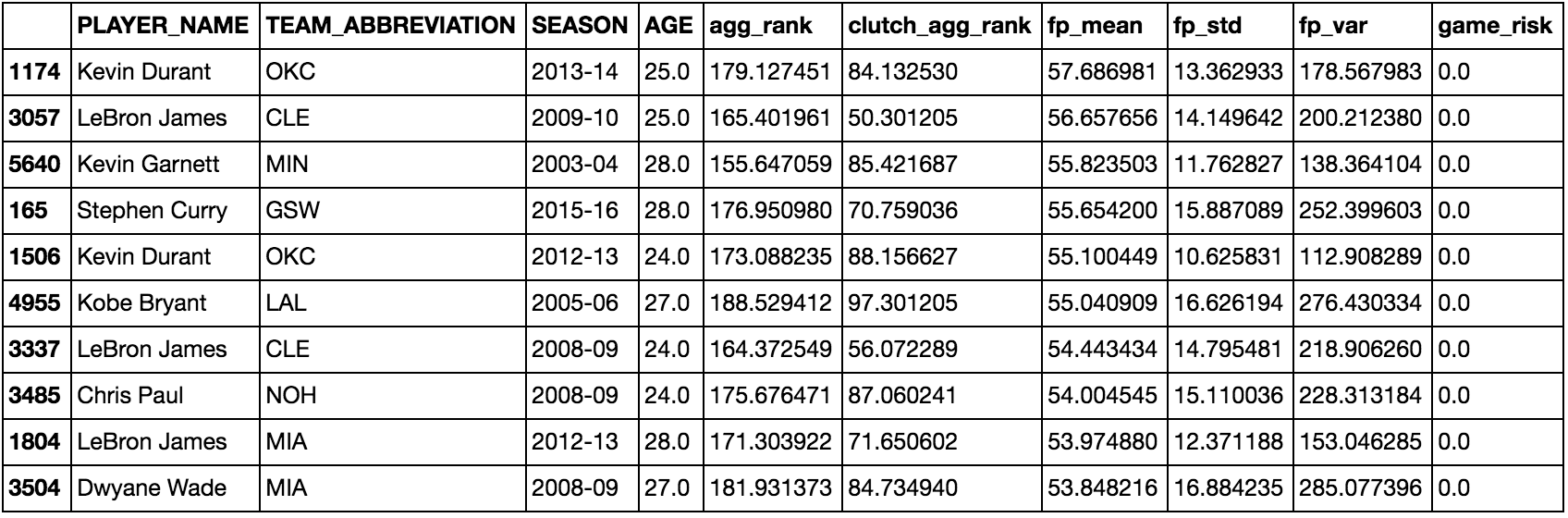
Top 10 Players with Combined all Target Dummy Variables
IV. EDA
Exploratory Data Analysis was very difficult because there is so much you can do with basketball data that you may lose direction and focus really easily. Before charging head first into EDA without any direction, I compiled a generic list of information that I was curious about related to fantasy. If my idea was not related to fantasy at all, I would dismiss it because not every information or idea that happens in real life on the court is translatable to getting more stats and winning your fantasy league. Below are the generic ideas I came up.
- Time series comparison between players
- Distribution of Fantasy Points
- Correlation Matrix between Targets
- Games Missed Risk Comparison
With these 4 points in mind, whenever I feel like I am getting lost or start thinking "what am I doing right now," I can refer back and get back on track.
Hall of Famers Fantasy Player by Median
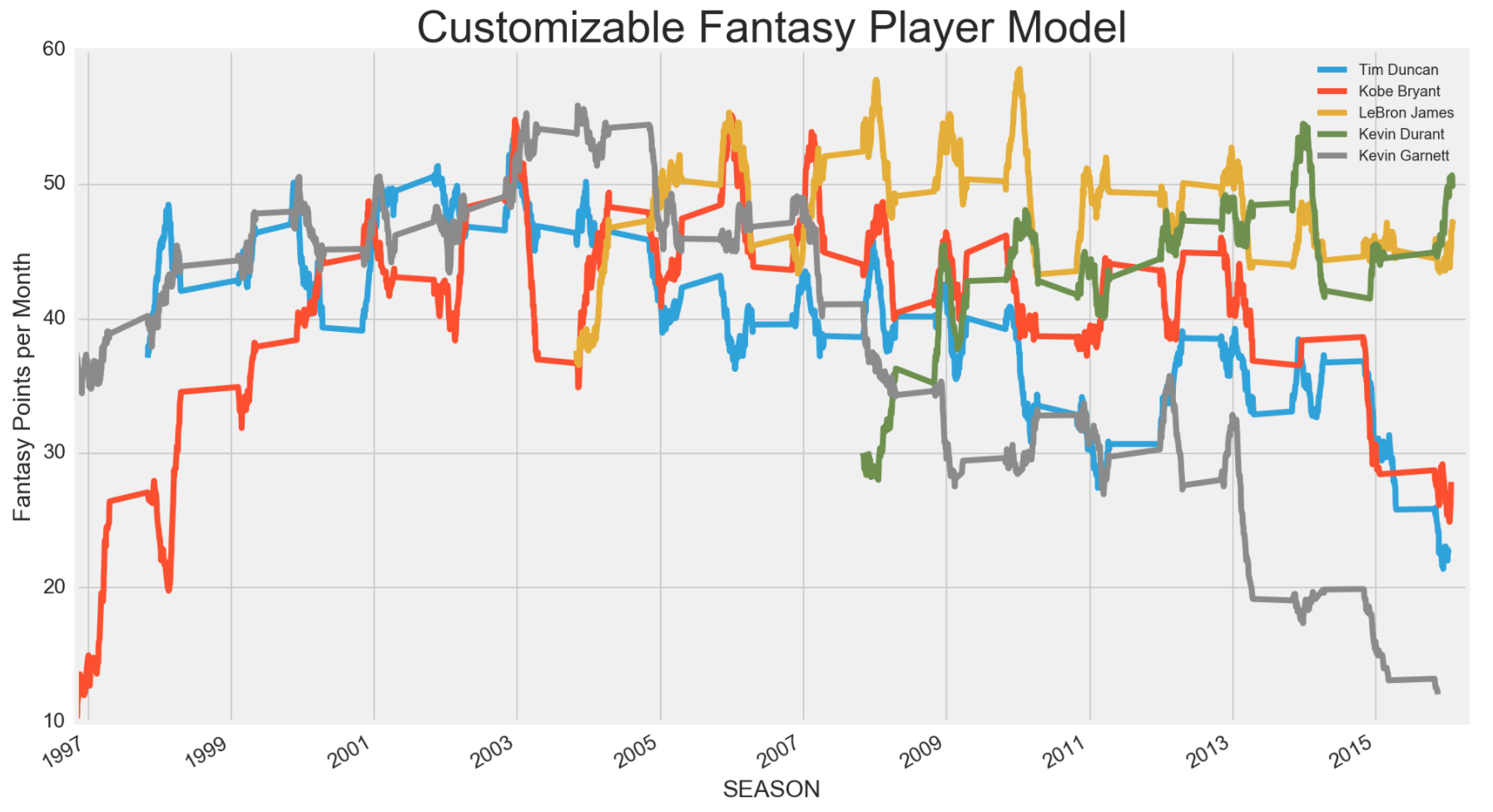
The above time series graph was one of the first graphs I made for fun, but sparked a bunch of ideas on how to use it. Initially, I just wanted to see the series on how the top tier players achieved through the whole career. Later I figured, I can compared players between different tiers, countries and draft rounds, which is what I did below.
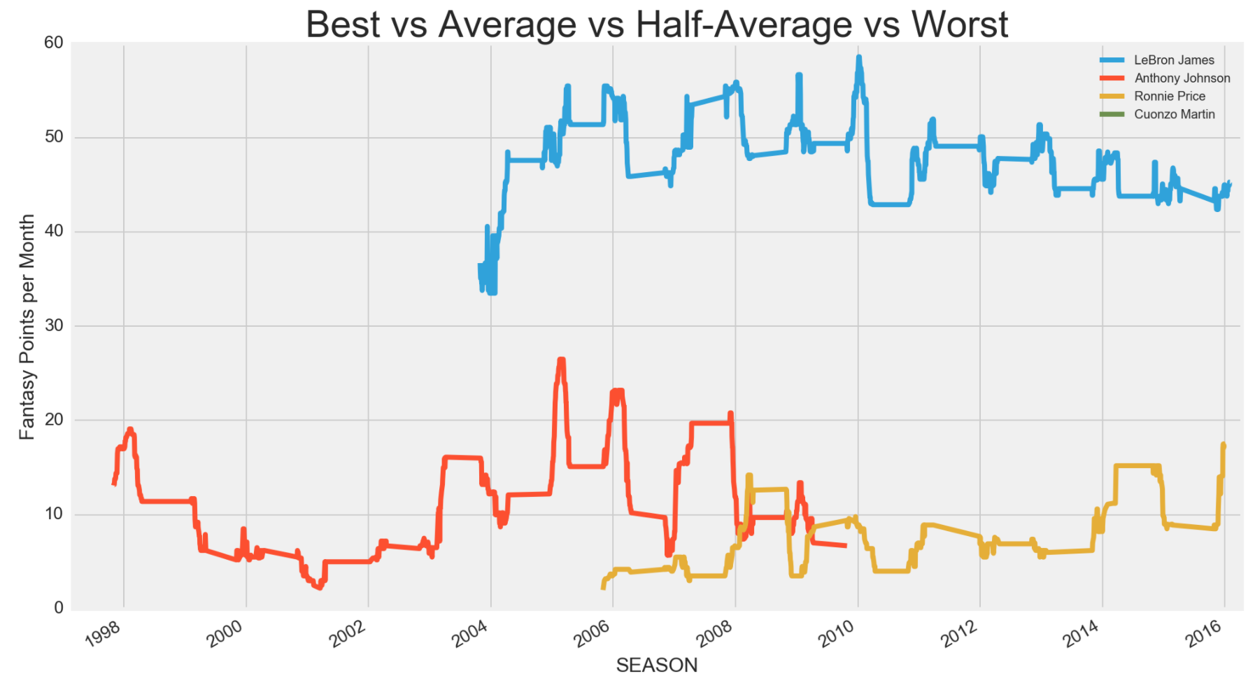
It is clear that LeBron James, being a top tier fantasy pick, was miles ahead of an average player. What was interesting was an average player like Anthony Johnson was not as good as I thought. Although he may have been one of the players at the median, Ronnie Price, who was half of the median (hence, half-average), was more consistent. I also did one for one of the players at the bottom 1st percentile and Cuonzo Martin did not show up on the graph at all. I wonder why until I plotted all the 1st percentile players below.
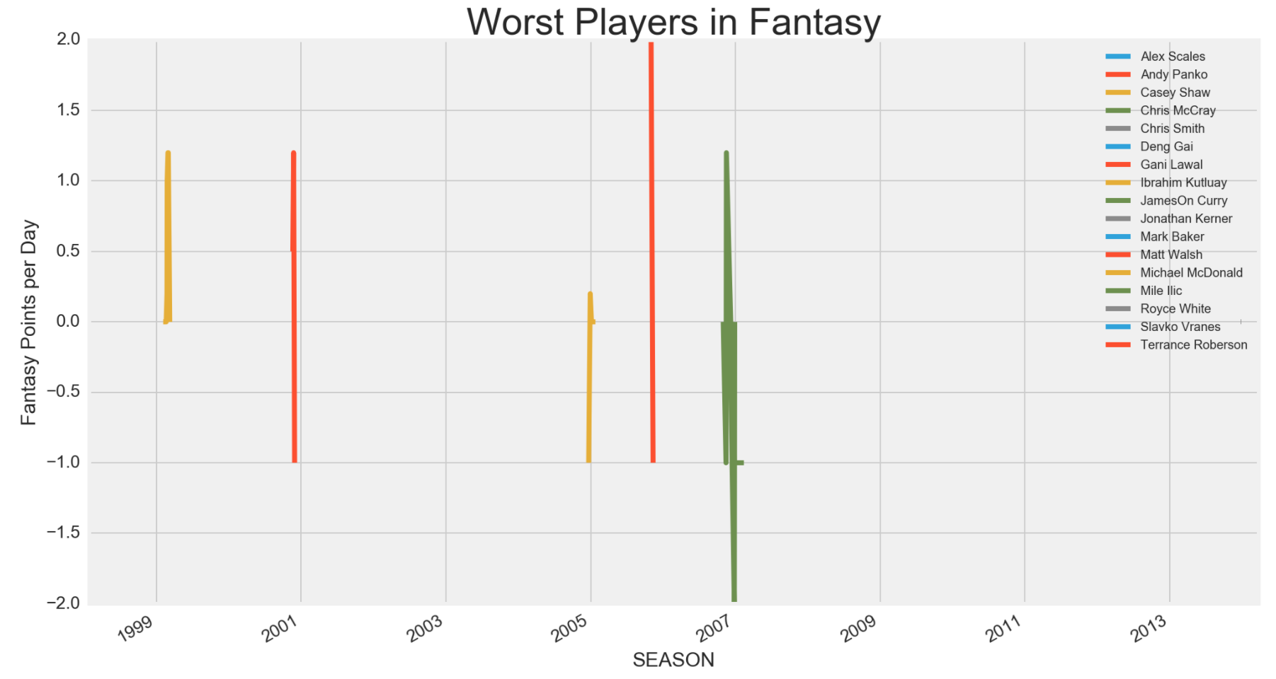
Most players who were at the bottom percentile were players that only played limited amount of games per season and were either cut or benched the rest of the season. I thought about subsetting them out, but even after subsetting, they did not affect my model much, so I just left them out when I was predicting for the upcoming season instead.
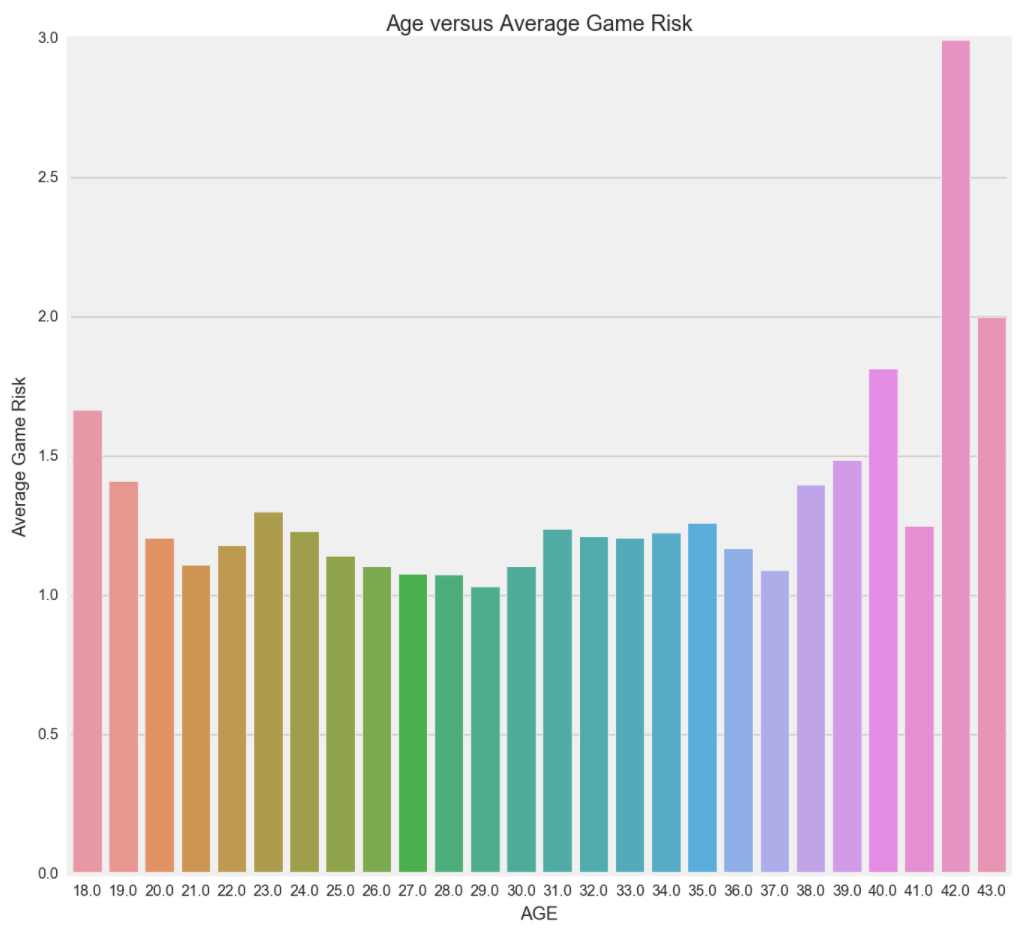
As experted, when you are younger or older, your game risk is higher. Most rookies don't get much playing time as many teams prefer to groom them off the court, while giving them some garbage time (blow out games) for experience. Rarely rookies get consistent playing time or play in every game. Older players have a higher game risk because they don't have the stamina and are more susceptible to injuries. Generally speaking, older players, also referred to as veterans, are usually there to help teach and bring confidence to the team's younger players. They don't play a lot of minutes and don't play every game, which is why their game risk is much higher.
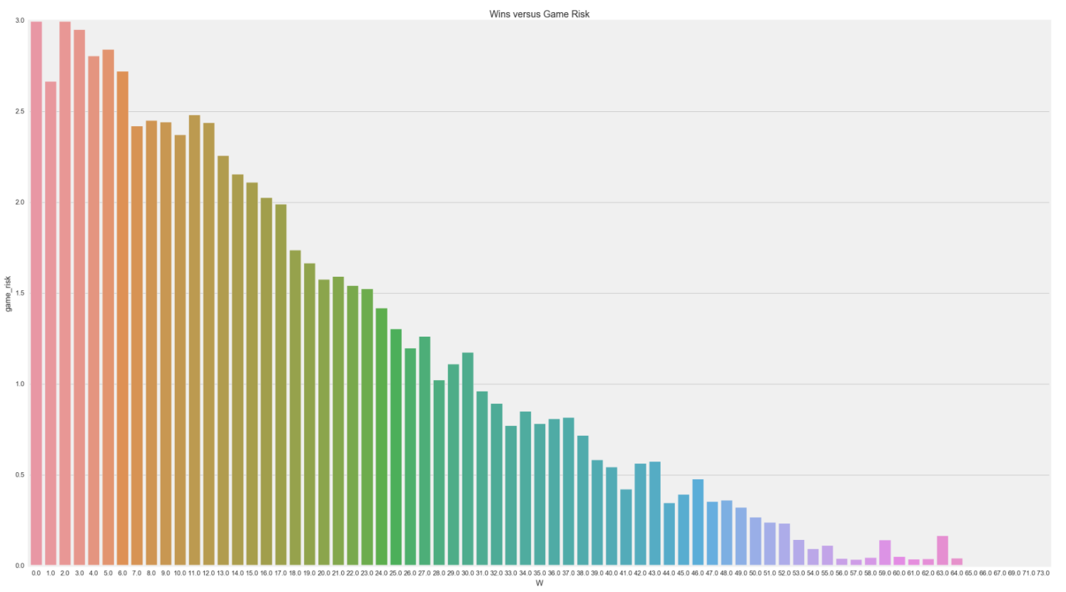
Also as expected with player's riskiness versus their wins. Players, who avoid injury risk, tend to be able to play more and stick to their team's game plan and output more wins.
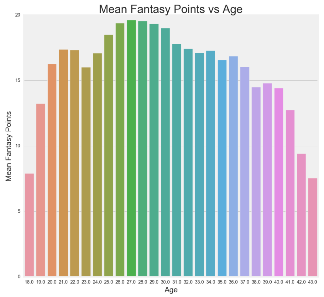
Players closer to their prime, roughly around 26-30, output higher average fantasy points. Another thing that is noteworthy is the increase from 18 to 22 and a decrease back to 23 before another increase. The reason is because in 2006, NBA set an age limit of 19, which is usually 1 year of college or 1 year playing overseas. The reason for the age limit is because mainly players, who are drafted out of high school, are more prone to bad decisions in life, especially if they do not pan out in the NBA. Players who leave college after 1 year, are represented by the first increase and players who leave after 4 years of college, are represented by the dip at the age 23 mark.
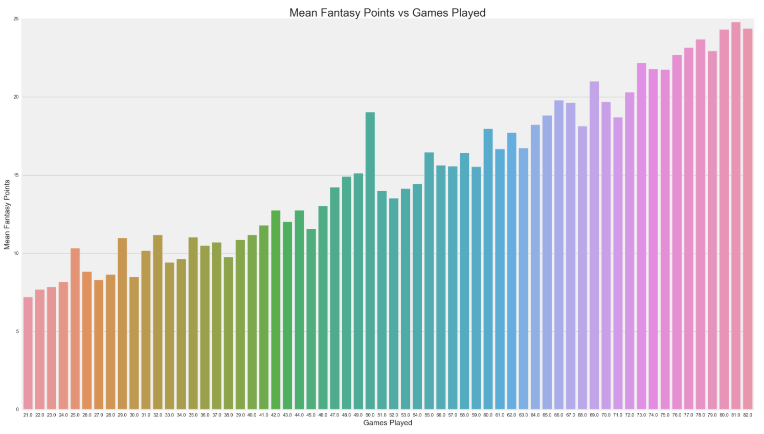
This is rather fun to look at. The more games a player plays, the higher their mean fantasy point output is. It makes sense because if you aren't performing well, you shouldn't be playing in so many games. Good players play at least 30 minutes per game and as many games as they are capable. What is interesting to me is the jump at 50 games played. For losing teams, 50 games seems to be the point where good players will stop the 82 game grind and start to take more rest days, especially if they are completely out of the playoff run or if they have a lingering injury.
I was always curious on how USA players' fantasy value differed from international players. Although international players are up and coming, I don't recall any strong candidate that was every picked early. I decided to compare USA and international players based on where they were drafted in the NBA draft and compare their fantasy values.
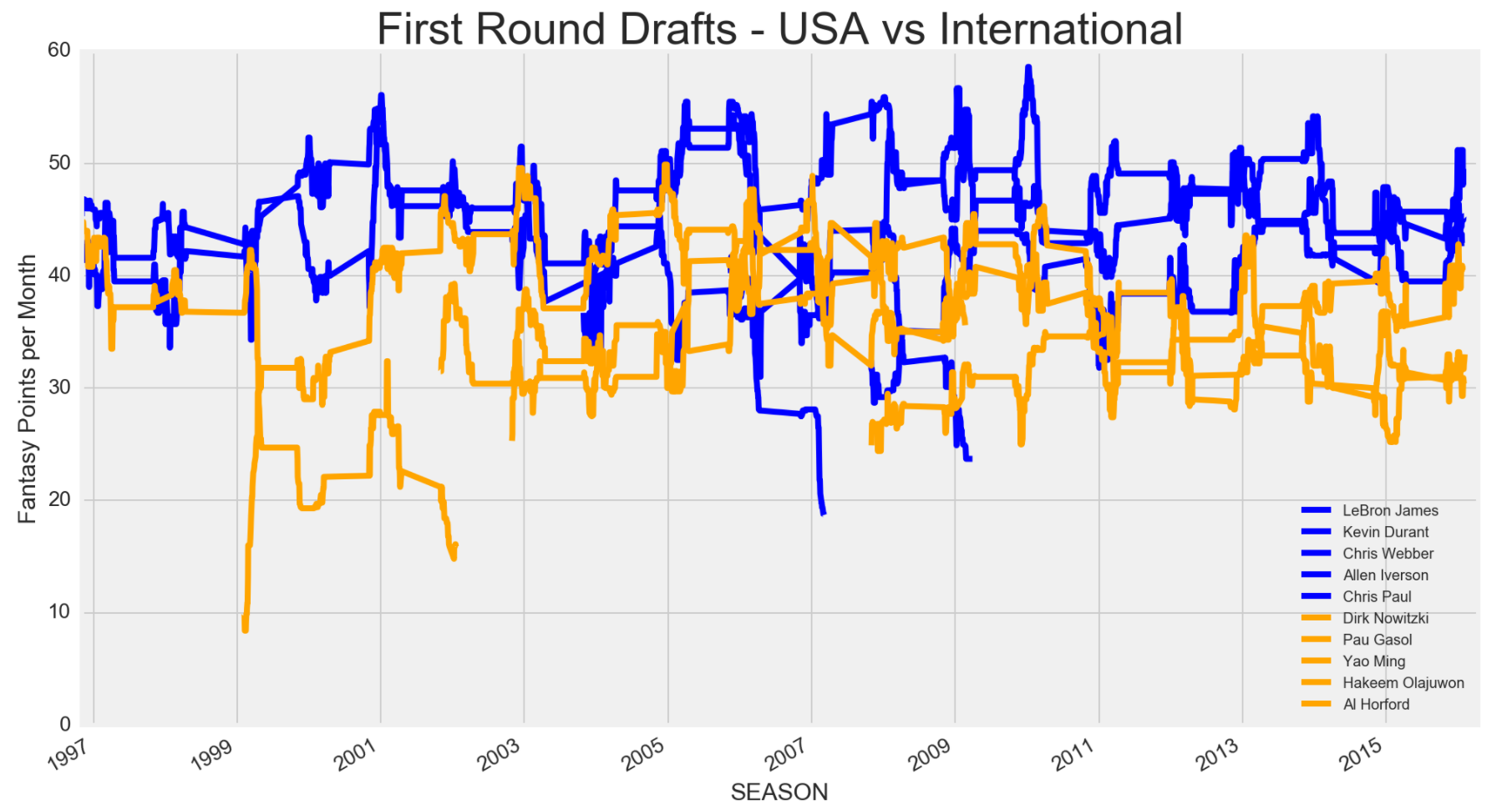
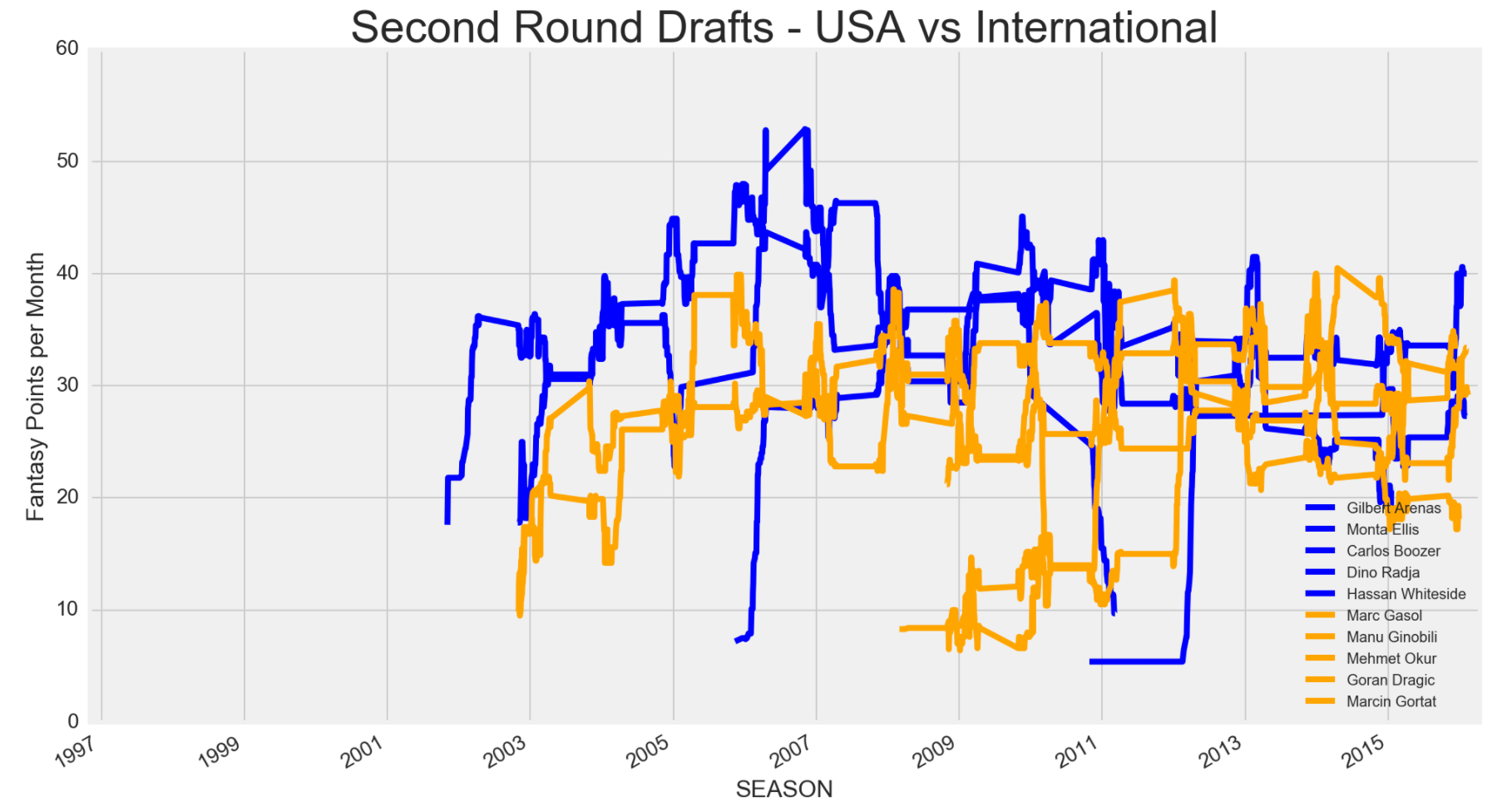
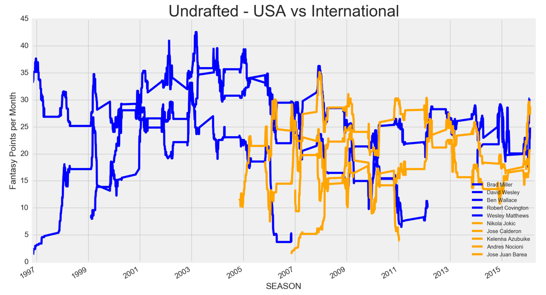
It looks pretty clearcut that in the past 20 seasons, the top 5 USA players drafted in the first round compared to the top 5 international players drafted in the first round were better fantasy players. However, starting from the 2005 season, international players in the 2nd round or undrafted, who were most likely being underrated, started to turn up to be on par with their USA counter parts. Currently, there are tons of NBA teams drafting more international players, so I wouldn't be surprised if international players in the future will be on par, fantasy wise, with USA players. Some international players not on the list, who were drafted in the first round and may become a fantasy studs include Kristaps Porzingis, Dario Saric, Mario Hezonja, Emmanuel Mudiay, Andrew Wiggins and Jusuf Nurkic.
Next, I wanted to see the density spread for fantasy points mean, standard deviation and variance. I expected that the 1st percentile to be closer to 0 based on what I found out earlier, but I also wanted to see how the rest of the distribution shaped out.
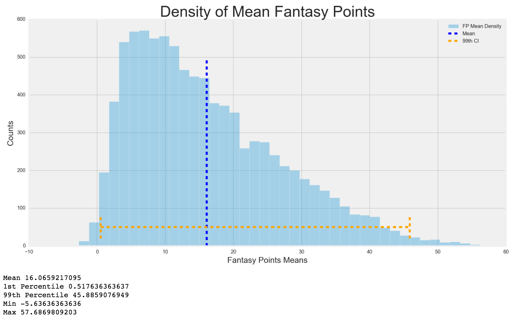
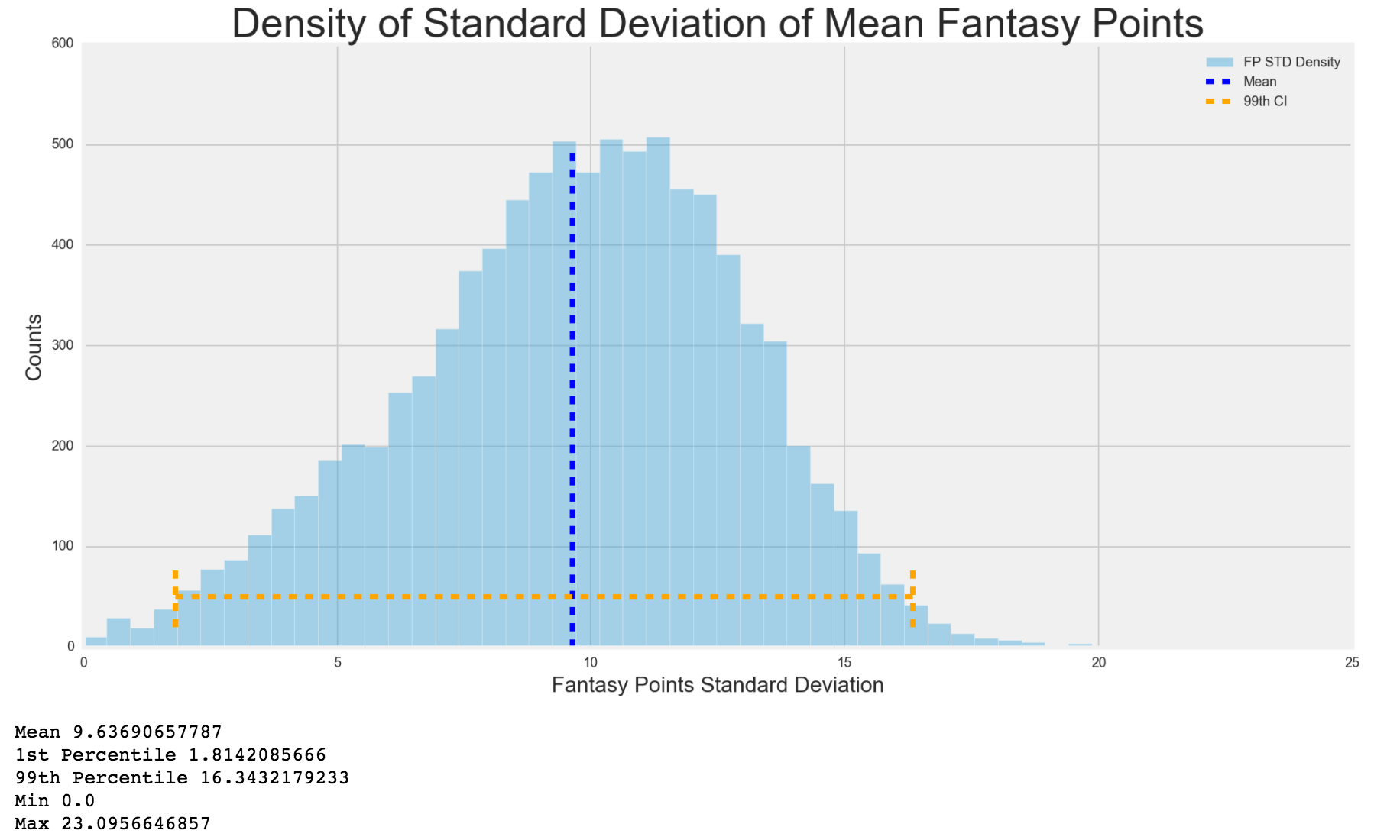
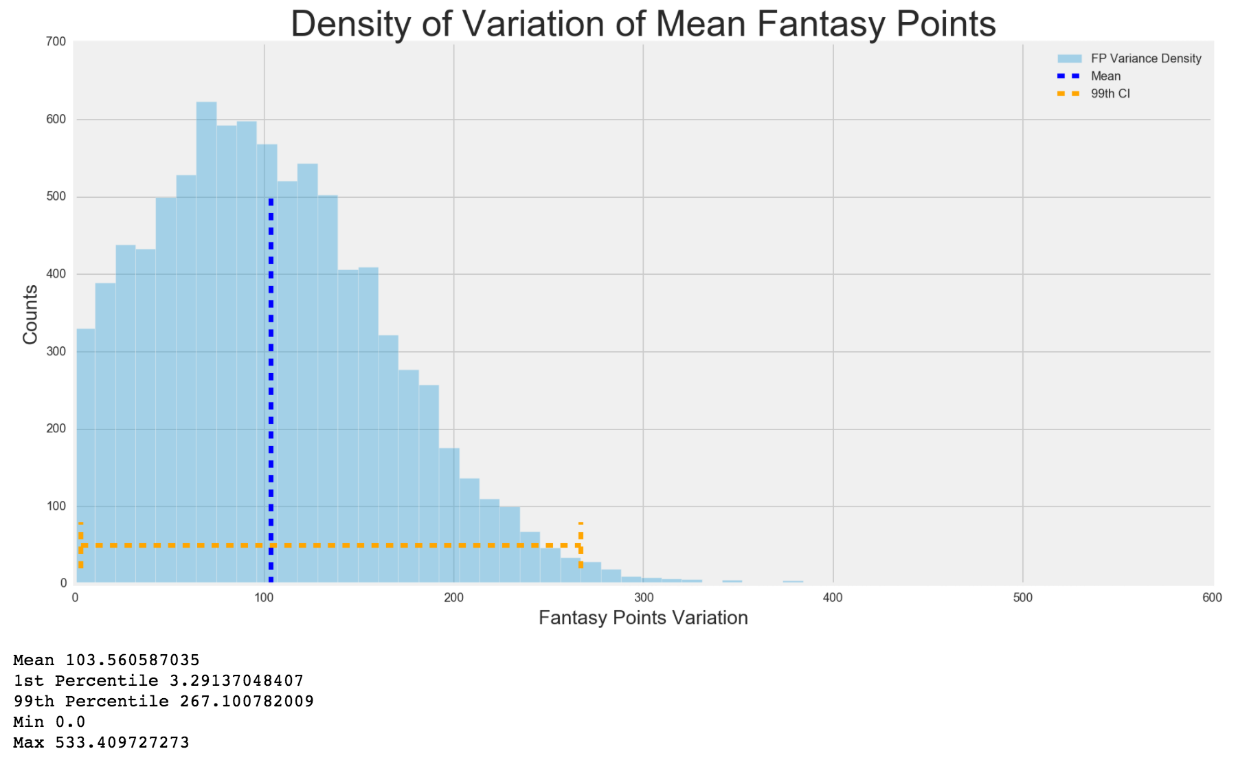
I must say, I was quite surprised at the results. I expected there to be a lot of values below the mean, but I did not expect so many players playing below the average. This just shows that in standard league, where you are only drafting 156 players, you are mostly drafting players way above the mean. It also shows how much of a fantasy monster the top 1st percentile are and how much they can affect a team. This also solidified my reasoning that less injury prone and consistent players should be emphasized on because you can't stand losing a fantasy monster to injury. The standard deviation and variance were normally distributed. I'd assume the ridicuously high variance players, which is creating a skewed right distribution, are players who played 2 games, one with a negative fantasy score and then another game with a high fantasy score.
Lastly, I wanted to make sure that my aggregate ranks were somewhat normally distributed and also that all my target variables were linearly correlated with each other.
![]()
![]()
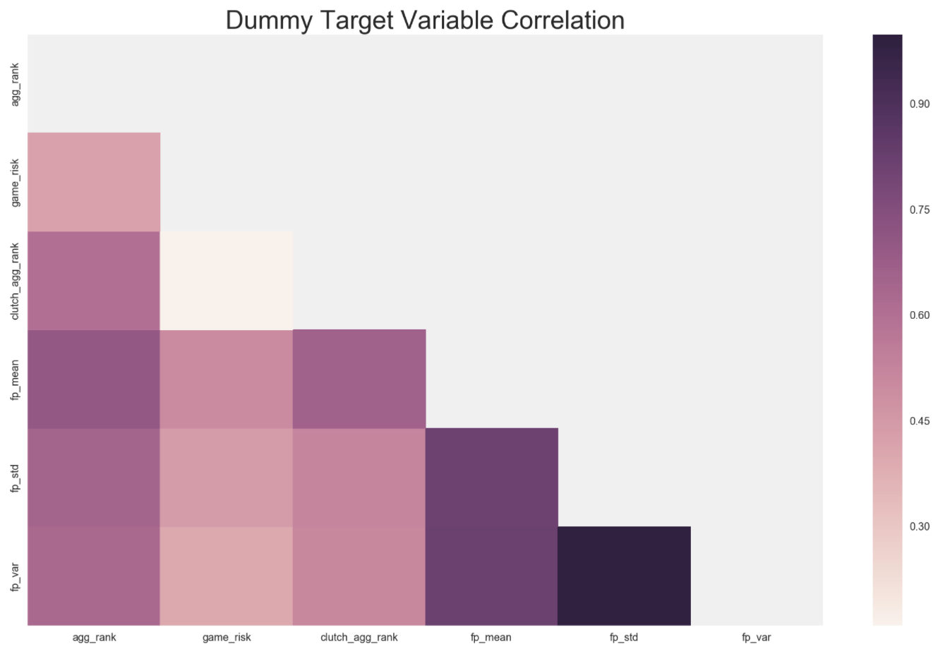
I was happy to see that all my dummy target variables I created were very correlated with each other. Clutch and game risk have close to 0 correlation, which is good because it makes sense. The higher the game risk, or games he can actually play, the less chance that player plays during the clutch.
V. Models
Linear/Logistic Regression vs Lasso vs Ridge vs Elastic Net
Basic Explanation of the Models
- Linear Regression - Linear Regression models how correlated your columns (predictors) are to your target.
- Lasso (aka L1) - Similar to Linear Regression, Lasso removes columns that it doesn't think will help the model, which creates a better model, but puts in more bias.
- Ridge (aka L2) - Similar to Linear Regression, Ridge tries to balance all the columns together so that they are equally affecting the best fit line. It tries its best not to remove any columns.
- Elastic Net - Elastic Net is a combination of both Lasso and Ridge. You can set the ratio between Lasso and Ridge to see if there is a possibility to not remove too many columns and also balance out the columns.
- Logistic Regression - Models the probability of an item being 1 thing or another. If there are 2 cats and 8 dogs, what is the possibility that the next animal brough in is a dog.
I used a Linear Regression for Aggregate Rank, Clutch Aggregate Rank, Fantasy Points Mean, Standard Deviation and Variance and a Logistic Regression for Games Missed Risk to look for any redundancy and correlation issues. In order to compare the results, I also ran a Lasso, Ridge and Elastic Net to see if there were any changes. Also, features such as 3Pt Made, 3Pt Attempted, Percentage of 3Pt Made, 20-24ft made from basket, etc... may all be redundant. It would be a good idea to figure out how the columns interacted with each other and understanding why before doing my Random Forest modeling.
Random Forests
Basic Explanation of Random Forests
Random Forest is an ensemble method for Decision Trees. Ensemble Method is running the same model, over and over again, and then averaging out all the scores for a more robust score. Decision Trees are like real trees. Imagine a real tree. As the tree starts growing, more branches and leaves are made. Now imagine that the stump is your entire data. Suppose that you are classifying whether 1 data point is a cat or dog. The Decision Tree will be like, dog - yes or no. If yes, go to this branch, if no, go to this other branch. Then in those branches it will ask a new question. Is it heavy - yes or no? If yes, go to this other branch, if no, go to this other branch. The Decision Tree will continue to ask questions until it decides, yes, this is a cat. Then it will identify this point as a cat. Random Forest is just a bunch of Decision Trees. This model is helpful for my project because it will help me classify whether this player is an allstar or a bench player by making decisions.
Random Forest Regressor and Classifier was my main modeling tool to predict my 2016-17 fantasy ranks. I chose Random Forest over Decision Trees because it was an ensemble method, which helped me test the strength of my dataset through bagging techniques. But the biggest reason I chose Random Forests was because it will help me categorize continuous variables into groups and split them, based on all my features, to determine a good player versus a bad player. I also figured, Random Forests will be able to help categorize the players in the 14 rounds I wanted to. I can create a new product, or ranking system, which I believe can beat Yahoo, ESPN, CBS and other ranking algorithms. If I wanted to improve my score, I would probably try and use Gradient Boosted Trees.
VI. Description of results.
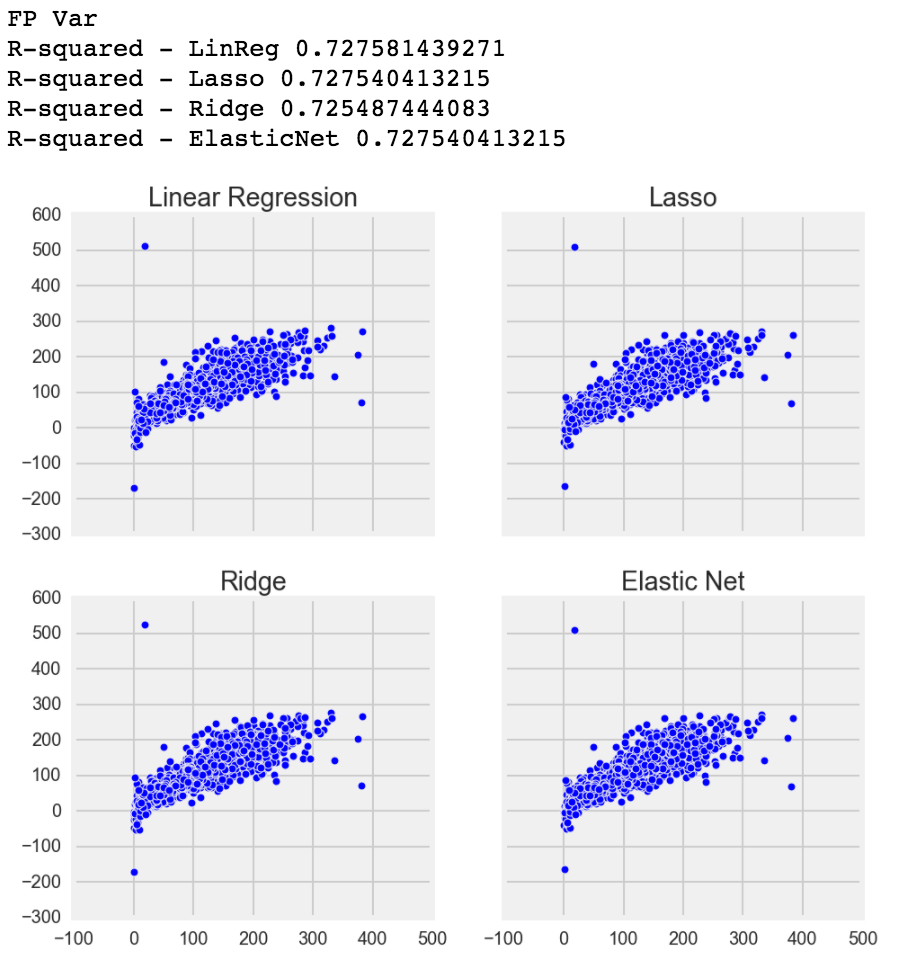
Linear, Logistic, Lasso, Ridge and Elastic Net Results
![]()
![]()
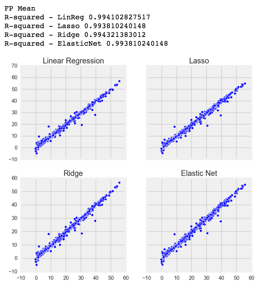
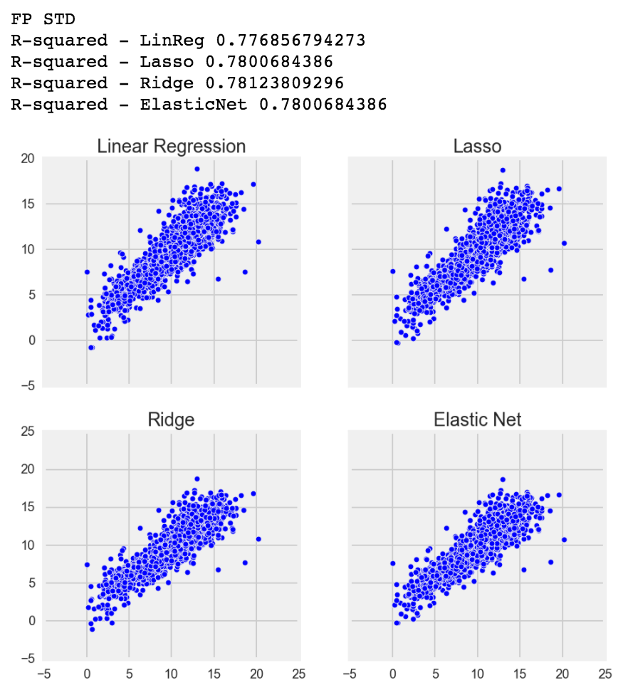
Before running Linear, Logistic, Lasso, Ridge and Elastic Net, I manually took out some columns that had 0 correlation with my target variables. Each target variable had different 0 correlations with each columns, so it took a long time to remove obvious redundancies.
However, after I ran my model, I was surprised that each target variable's Linear Regression, Lasso, Ridge and Elastic Net were very similar to each other, and my Elastic Net L1/2 ratio (the ratio and balance between the model using Lasso and Ridge) always used full Lasso over Ridge. I was fairly surprised that my fantasy points mean had an R-squared of 0.99+! R-squared can be thought of how close each point, when compared to the target variable, is to the best fit line. The closer the points are to the line, the higher the R-squared. If R-squared is 0.0, that indicates that the model does not explain any of the variability of the data and guessing what the value would be is as good as the model.
Although only using the basic 9 categories of FGM/FGA, FTM/FTA, 3PTM, Points, Rebounds, Assists, Steals, Blocks and Turnovers, every single column was positively linearly correlated (positive is when 1 variable goes up, the other variable will go up as well, negative would be when 1 variable goes up, the other simultaneously goes down). However, there may be still some multicollinearity, but I don't think it's a bad thing. Multicollinearity is when 2 or more columns are so correlated that one column can predict the other column at a high accuracy. This may be a problem where the R-squared increases when it shouldn't. However, I doubt removing those features will vastly affect my score because the columns are all good predictors to my dummy targets, so at this point I was ready to move onto Random Forests.
Logistic Regression Confusion Matrix
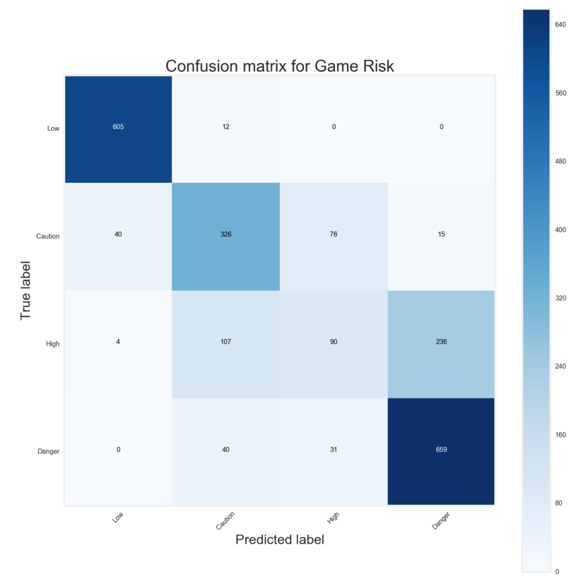
The confusion matrix is to detect how many True Positive, False Positive, True Negative and False Negative there are when my model is predicting if the player is more injury prone or not.
- True Positive - Model predicted positive correctly and in actuality, it is positive.
- False Positive - Model predicted positive incorrectly and in actuality, it is negative.
- True Negative - Model predicted negative correctly and in actuality, it is negative.
- False Negative - Model predicted negative incorrectly and in actuality, it is positive.
Confusion matrix is extremely important because if a player was predicted to be very healthy, but the model predicted him to be extremely not healthy, people drafted would be avoiding a very good player rather than picking him up. The logistic regression confusion matrix did very well predicting low and danger risk players. It also did pretty good on caution. However, high risk players (missing 25-50% games) performed extremely poorly. The model had trouble differentiating between caution, high and danger players, which is interesting. It does seem that players who have high risk (203) tend to lean towards danger, while some (122) leaning towards caution. As noted in the caution predicting 75 as high, it might be better to create 3 brackets instead of 4. However, I want to see how my random forest classifier performs before deciding whether to go with 3 or 4 brackets.
Logistic Regression ROC/AUC
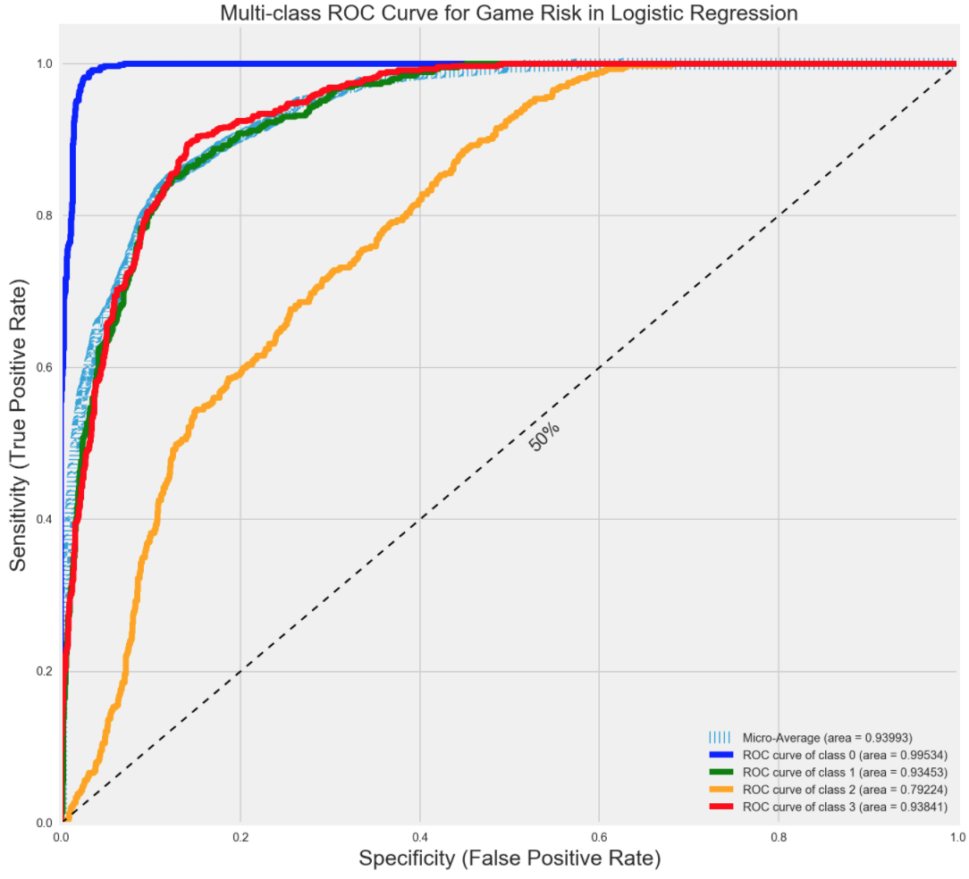
The ROC curve (Receiver Operating Characteristic) is a chart that plots the True Positives over the False Positives. The point of the curve is to make sure that when your model is predicting if it is yes or no, at what probability rate is the model predicting yes and it actually is yes, and no when it is actually yes. The diagonal line is the baseline, where guess would be the same probability. Below the line is your model guessing no more, when it is actually yes.
As noted before, low, caution and danger risk players perform well and high, although overall it seems to have predicted more true positives than false negatives, did not perform that well.
Logistic Regression Classification Report
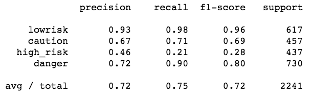
Precision is when the model predicts yes, how often is it correct. Recall is how often the model predicts yes, and it is actually yes. F1-score is the weighted average between precision and recall, where 0 is bad and 1 is good. Both precision and recall were not great, there were more false negative and false positives than true positives and true negatives. The higher the value, the better the predictor is at guessing correctly. As mentioned before, this may be interesting to see if it can be tweaked a bit more, such as moving to 3 classes instead of 4, but I wanted to see how my Random Forest performed in comparison to my logistic regression.
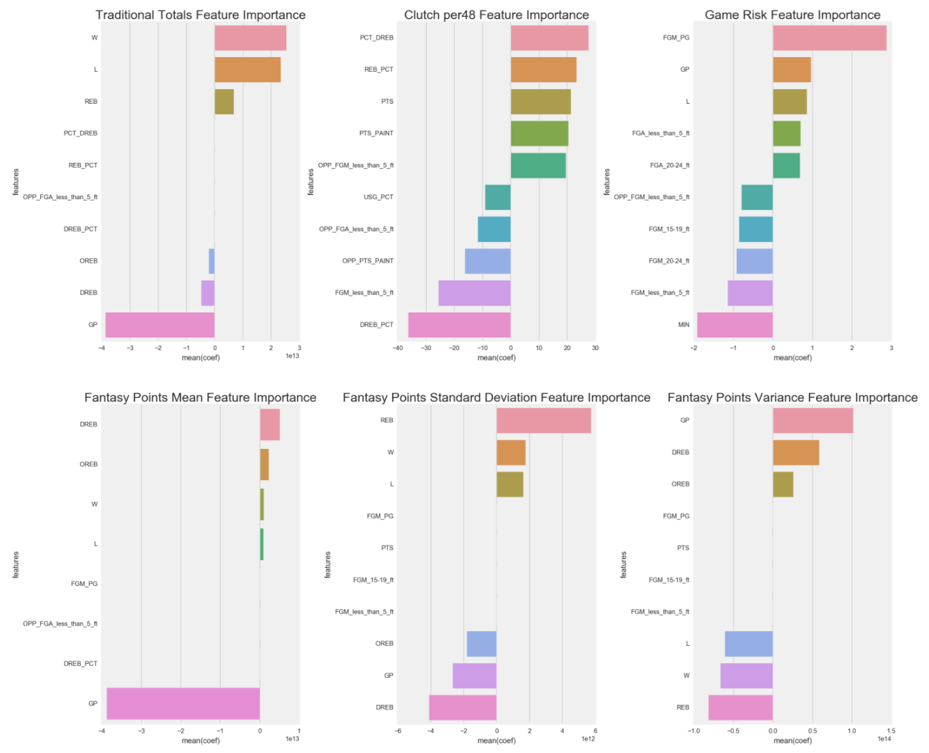
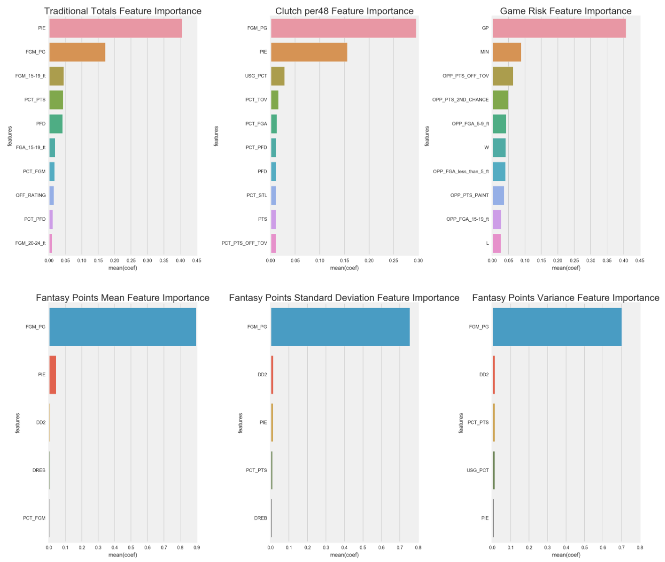
Linear/Logistic Regression Feature Importance
Feature importance is an analysis method to see which features are the highest influences to the predictive model, both positively and negatively.
However, the results show that I need to do more feature engineering to figure out collinearity. For example, Traditional Totals Feature Importance has Wins and Losses as a positive influence, while GP (games played) as a negative influence, which means they are just cancelling each other out. Same with DREB (defensive rebounds) and OREB (offensive rebounds) being negative influences, while REB (total rebounds) being a positive influence.
Some features do make sense, such as Clutch per48's PCT_DREB, REB_PCT, PTS and PTS_PAINT. Players who play better defense, causing more missed shots and increasing rebounds, while also scoring a lot of points, and especially points in the paint, are more likely to perform better during the clutch period.
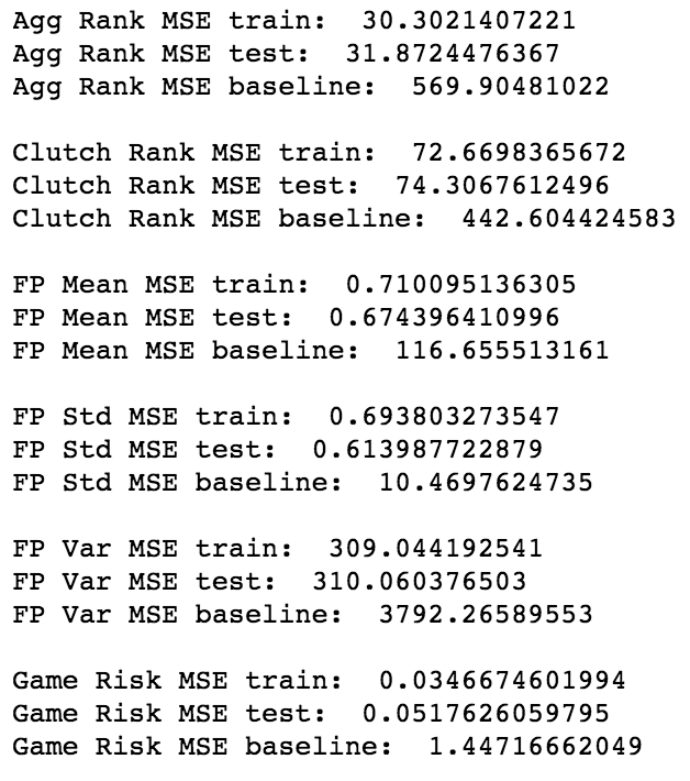
Random Forest Results
Random Forest Mean Squared Error
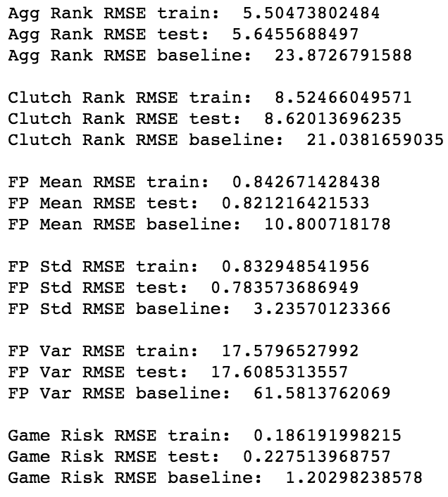
Random Forest Residual Mean Squared Error
Random Forest R-Squared
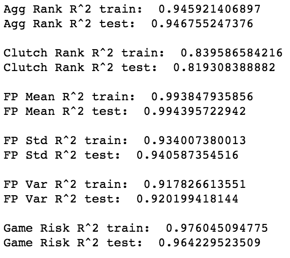
My Random Forest performed exceptionally well for their Mean Squared Error, Residual Mean Squared Error and R^2. They are all far superior than their average (baseline) and much better than the performance than Linear/Logistic Regression, Lasso, Ridge and Elastic Net.
Confusion Matrix
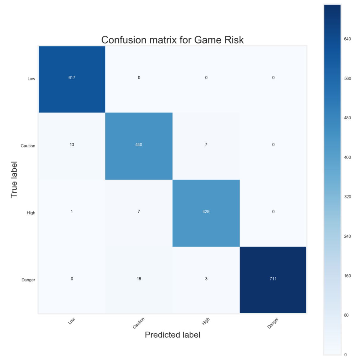
My random forest classifier for games missed risk performed extremely well, much better than my logistic regression. The model was able to correctly predict all 4 brackets extremely accurate.
Random Forest ROC/AUC
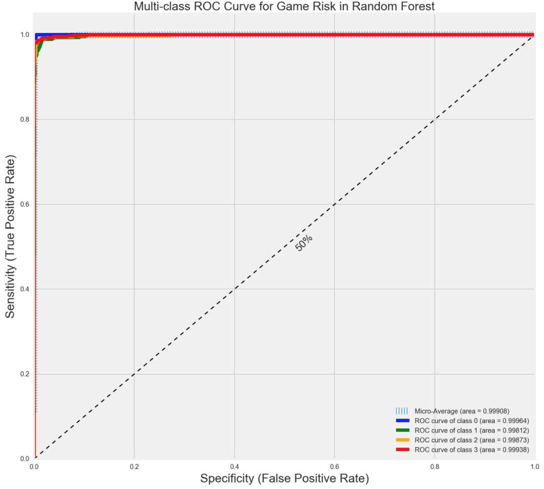
My ROC/AUC also showed a near perfection of being correct.
Random Forest Classification Report
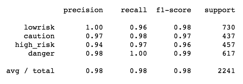
Makes sense that my precision, recall and f1-score are all much better compared to my logistic regression.
Random Forest Feature Importance
Here are the feature importances below.
It is noteworthy that multicollinearity does not affect features influences since the model has a different decision to make after each node.
- FGM_PG (Field Goal Made per Game)
- Traditional Totals: As a player makes more field goals per game, the more likely he'll be in the game (more minutes) impacting the game.
- Clutch per48: During clutch time, a player who makes more FGM_PG, the more clutch he is.
- Fantasy Points Mean: Players who score more, tend to output more fantasy points.
- Fantasy Points Standard Deviation: Players who score more, tend to have a lower standard deviation.
- Fantasy Points Variance: Players who score more, tend to have a lower variance.
- PIE (Player Impact Estimate)
- Traditional Totals: A player who impacts and influences the game more will produce more stats.
- Clutch per48: A player who impacts and influences the game will be more clutch.
- GP (games played)
- Games Risk: The more games a player plays, the higher the probability that player gets injured.
- MIN (Minutes)
- Games Risk: The more minutes a player plays, the higher the probability that player gets injured.
VII. Conclusion
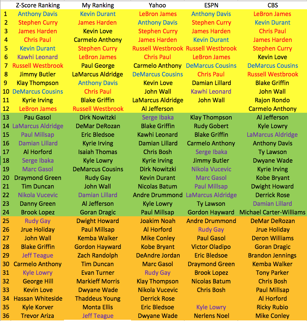
Pure Z-Score Ranking vs ALL
I compared the ranks from BasketballMonster.com, who uses Z-Score for each category and then aggregates each category by their algorithm, as the base for comparison. I used BasketballMonster.com as the base because it is the most basic and unbiased ranking system based on every player's standard 9 categories performance. I could only compare the past 2 seasons because past original ranking data for each big website was not always available. As my original goal stated, I wanted to do buckets, so instead of comparing rank by rank, I compared the first 3 round buckets.
2014-15 Season Ranking Comparisons
ESPN had the most accurate predictions with 16 correct in 3 rounds (44% accuracy), while my ranking tied with Yahoo and CBS with 9 correct in 3 rounds (25% accuracy).
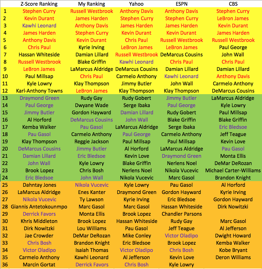
2015-16 Season Ranking Comparisons
My ranking did the best in this season with 14 correct in 3 rounds (38.89%), Yahoo and ESPN tied with 13 correct in 3 rounds (36.11%) and CBS had, by far, the worst original rank with 9 correct in 3 rounds (25%).
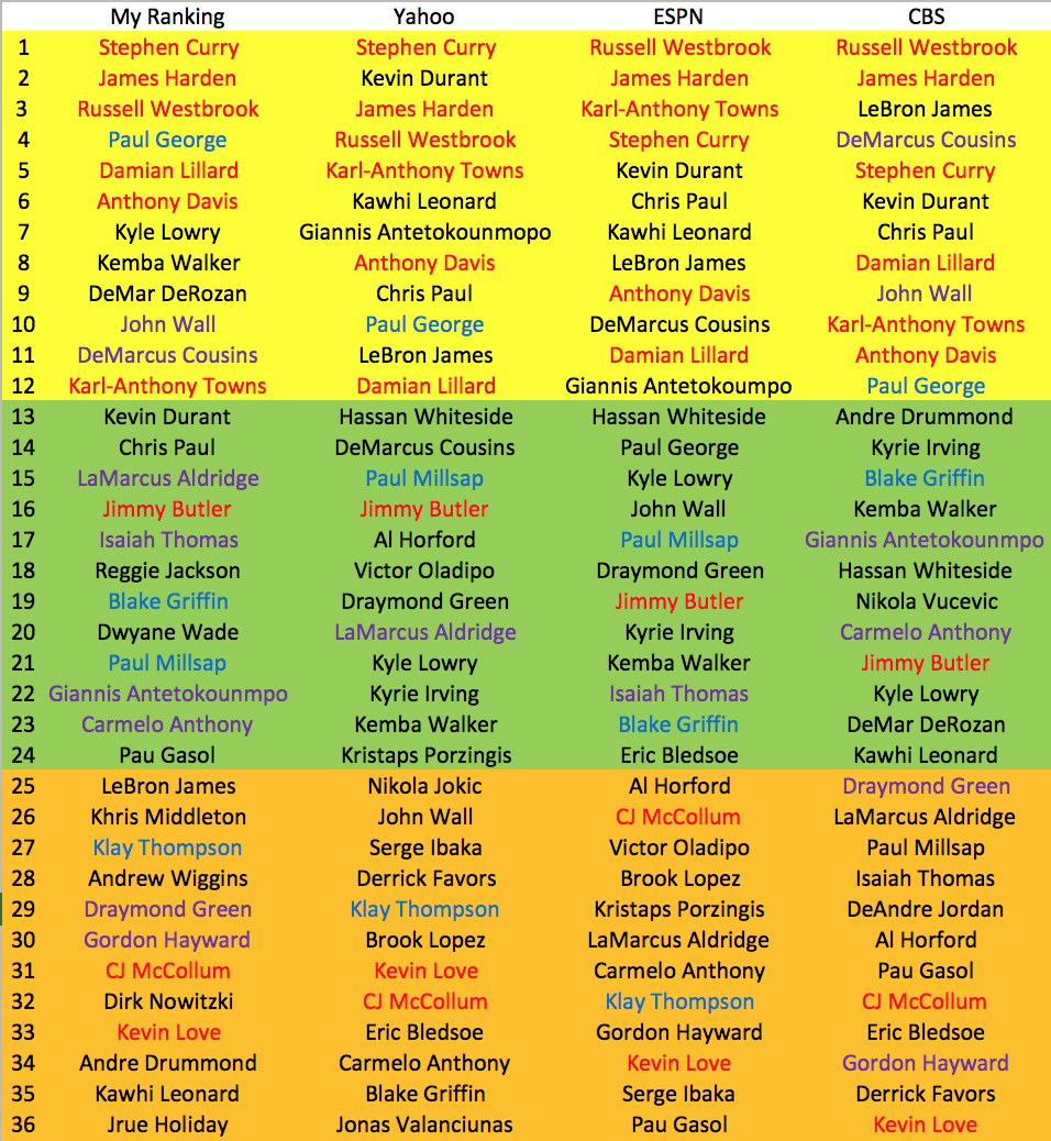
2016-17 Season Ranking Comparisons
Since this is the current season, there isn't a base Z-Score I could use to compare the ranks. Instead, I compared my ranks with each of the other websites to see the similarities and differences. CBS has the most similarities with my ranking, while Yahoo and ESPN tied with the same amount of similar rankings as mine. CBS does seem to have performed the worst, based off of the last 2 seasons, but because CBS didn't supply original rankings past 2 seasons ago, I could not see whether or not they performed better in the past. Although based off of my experience, I'm fairly confident that my ranking system does seem rather logical, but will have to see how I fare at the end of the season.
Based off of the last 2 seasons, CBS does seem to have the worst Z-Score ranking, while ESPN had the best performance. Yahoo and my ranking are similar, but mine performing slightly better. I am not sure how ESPN is obtaining such a high score because some of the ranking system does not make much sense and does not seem to be their "original" preseason rank. However, I do have each websites "original" rank for the 2016-17 season, so we will see how they really fared.
Below is my full 13 rounds, 12 players per round, bucket system.
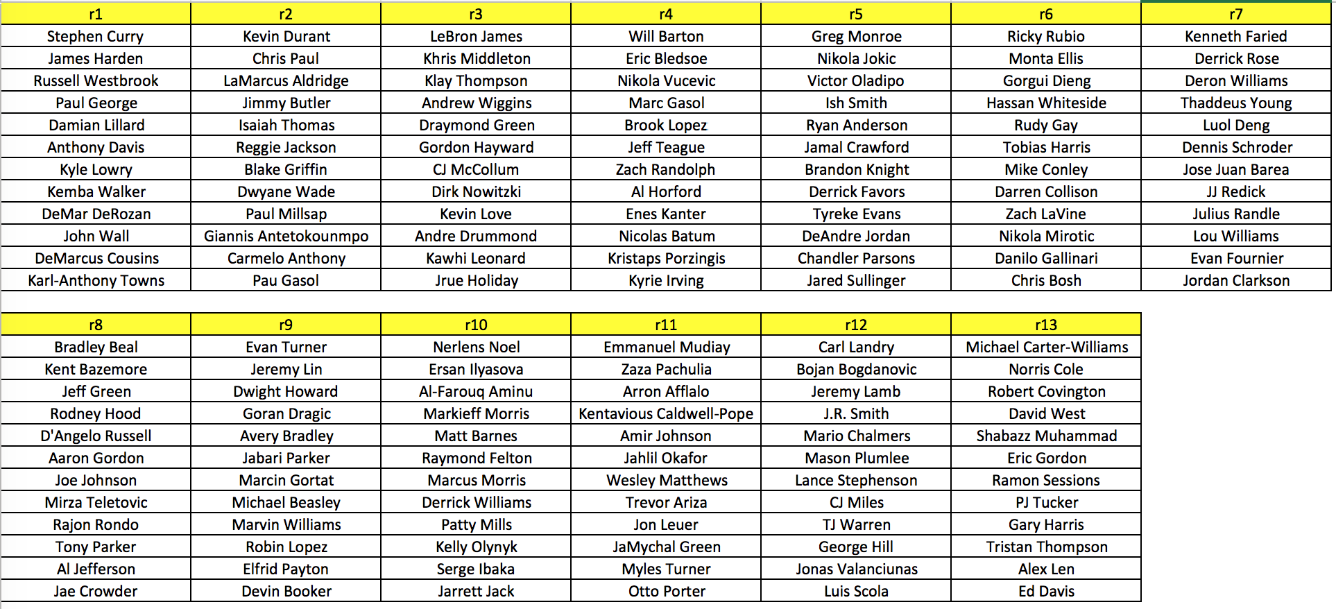
There is no way to justify whether or not my predictions are correct or not until the end of the season, but based off of experience alone, there are a couple of hiccups. First off, DeMar DeRozan should not be drafted in the first round and Kevin Durant should be in the first round. However, DeMar DeRozan may do well and explode this season for fantasy, so my algorithm may be correct. Overall, it does seem relatively good. I would definitely follow this ranking system for my next fantasy draft to test it out on first hand.
Next Step
This project still has a ton of possibilities to work with. Here are a couple of things I would definitely do to try and improve my projects.
- Figure out some way to tweak the weights to help update the model.
- Find a better way to combine all the predicted target values together to weight the ranks better.
- Subset the entire dataframe again to remove all the players who played less than a certain amount of games and rerun all my models
- Research more possible target dummy variables
- Maybe do a cluster to see what happens
Overall, I will continue to work on this project, but not day-to-day. I'm interested to wait for the end of the season to see how well my predicted ranks actually did. Depending on how well my model worked, I can tweak my models better.